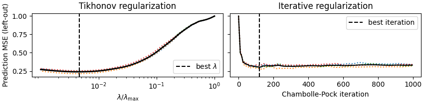
Plot Chambolle Pock path vs Lasso Tikhonov path

Comparison of Tikhonov regularization path (fast LassoCV with the celer package) and iterative regularization (ours).

import time
import numpy as np
import matplotlib.pyplot as plt

from scipy import sparse
from celer import LassoCV
from numpy.linalg import norm
from libsvmdata import fetch_libsvm
from sklearn.model_selection import KFold
from joblib import Parallel, delayed

from iterreg.sparse import dual_primal
from iterreg.sparse.estimators import SparseIterReg


dataset = 'rcv1.binary'
X, y = fetch_libsvm(dataset)
# make dataset smaller for faster example:
X = X[:5000]
y = y[:5000]

n_splits = 4
kf = KFold(n_splits=n_splits, shuffle=True, random_state=0)

clf = LassoCV(fit_intercept=False, n_jobs=4, cv=kf, verbose=0)

clf.fit(X, y)

max_iter = 1_000
f_store = 5
L = sparse.linalg.svds(X, k=1)[1][0]
sigma_good = 1. / norm(X.T @ y, ord=np.inf)
step_ratio = 0.99 / (L ** 2 * sigma_good ** 2)
n_points = max_iter // f_store
mse_dp = np.zeros((n_points, n_splits))

res = Parallel(n_jobs=-1)(delayed(dual_primal)(
    X[train_idx], y[train_idx], step_ratio=step_ratio, max_iter=max_iter,
    f_store=f_store, verbose=True)
    for train_idx, _ in kf.split(X))
all_w = np.array([result[-1] for result in res])

for split, (train_idx, test_idx) in enumerate(kf.split(X)):
    mse_dp[:, split] = np.mean(
        (X[test_idx] @ all_w[split].T - y[test_idx, None]) ** 2, axis=0)


best_alpha = clf.alpha_

plt.close('all')
fig, axarr = plt.subplots(
    1, 2, sharey=True, figsize=(8.5, 2.1), constrained_layout=True)
ax = axarr[0]
ax.semilogx(clf.alphas_ / clf.alphas_[0], clf.mse_path_, ':')
ax.semilogx(clf.alphas_ / clf.alphas_[0], clf.mse_path_.mean(axis=-1), 'k',
            linewidth=2)
ax.axvline(clf.alpha_ / clf.alphas_[0], linestyle='--', color='k',
           label=r'best $\lambda$')

ax.set_title("Tikhonov regularization")
ax.set_xticks([1e-2, 1e-1, 1e0])

ax.set_xlabel(r'$\lambda / \lambda_{\mathrm{\max}}$')
ax.set_ylabel('Prediction MSE (left-out)')
ax.legend()

ax = axarr[-1]
ax.set_title("Iterative regularization")
ax.plot(f_store * np.arange(n_points), mse_dp, ':')
ax.plot(f_store * np.arange(n_points), mse_dp.mean(axis=-1), 'k')
best_iter = f_store * np.argmin(np.mean(mse_dp, axis=-1))
ax.axvline(best_iter, linestyle='--', color='k', label='best iteration')
ax.set_xlabel("Chambolle-Pock iteration")
ax.legend()

plt.show(block=False)

Out:

Dataset: rcv1.binary
Downloading data from https://www.csie.ntu.edu.tw/~cjlin/libsvmtools/datasets/binary/rcv1_train.binary.bz2 (13.1 MB)


file_sizes:   0%|                                   | 0.00/13.7M [00:00<?, ?B/s]
file_sizes:   0%|                           | 24.6k/13.7M [00:00<01:48, 126kB/s]
file_sizes:   0%|                           | 49.2k/13.7M [00:00<01:49, 125kB/s]
file_sizes:   1%|2                           | 106k/13.7M [00:00<01:07, 201kB/s]
file_sizes:   2%|4                           | 221k/13.7M [00:00<00:38, 352kB/s]
file_sizes:   3%|9                           | 451k/13.7M [00:00<00:20, 645kB/s]
file_sizes:   7%|#7                         | 909k/13.7M [00:01<00:10, 1.22MB/s]
file_sizes:  13%|###4                      | 1.83M/13.7M [00:01<00:05, 2.34MB/s]
file_sizes:  27%|######9                   | 3.66M/13.7M [00:01<00:02, 4.53MB/s]
file_sizes:  38%|#########9                | 5.23M/13.7M [00:01<00:01, 5.60MB/s]
file_sizes:  50%|############8             | 6.81M/13.7M [00:01<00:01, 6.33MB/s]
file_sizes:  61%|###############8          | 8.38M/13.7M [00:02<00:00, 6.83MB/s]
file_sizes:  72%|##################8       | 9.95M/13.7M [00:02<00:00, 7.18MB/s]
file_sizes:  84%|#####################8    | 11.5M/13.7M [00:02<00:00, 7.42MB/s]
file_sizes:  95%|########################8 | 13.1M/13.7M [00:02<00:00, 7.58MB/s]
file_sizes: 100%|##########################| 13.7M/13.7M [00:02<00:00, 4.96MB/s]
Successfully downloaded file to /home/circleci/celer_data/libsvm/binary/rcv1_train.binary.bz2
Decompressing...
Loading svmlight file...

Now do the timings a posteriori, as if we knew the optimal iteration/lambda

bp = SparseIterReg(max_iter=best_iter, memory=best_iter + 1,
                   step_ratio=step_ratio)
t0 = time.perf_counter()
bp.fit(X, y)
time_cp = time.perf_counter() - t0
print("Duration for CP: %.3fs" % time_cp)

# default grid:
alpha_max = np.max(np.abs(X.T @ y)) / len(y)
alphas = np.geomspace(1, 1e-3, 100) * alpha_max
alphas_stop = alphas[alphas >= best_alpha]

# time if we stopped at best_alpha:
t0 = time.perf_counter()
clf2 = LassoCV(fit_intercept=False, alphas=alphas_stop,
               verbose=0, cv=4, n_jobs=4).fit(X, y)
time_cv = time.perf_counter() - t0


print("CP early stop needs %d iter" % best_iter)
print("LassoCV optimal lambda: %.2e lambda_max" %
      (best_alpha / clf2.alphas_[0]))
print("CP time: %.3f s" % time_cp)
print("CV time: %.3f s" % time_cv)
print("CP support size: %d" % (bp.coef_ != 0).sum())
print("CV support size: %d" % (clf.coef_ != 0).sum())

Out:

Duration for CP: 0.676s
CP early stop needs 120 iter
LassoCV optimal lambda: 4.64e-03 lambda_max
CP time: 0.676 s
CV time: 11.574 s
CP support size: 714
CV support size: 1430