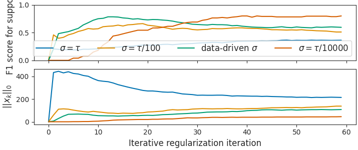
Data-driven for dual stepsize choice in sparse recovery

From the data, a good dual stepsize can be estimated in the case of sparse recovery.

import numpy as np
from numpy.linalg import norm
import matplotlib.pyplot as plt
from sklearn.metrics import f1_score
from celer.datasets import make_correlated_data
from celer.plot_utils import configure_plt

from iterreg.sparse import dual_primal

configure_plt()

# data for the experiment:
n_samples = 200
n_features = 500

X, y, w_true = make_correlated_data(
    n_samples=n_samples, n_features=n_features,
    corr=0.2, density=0.1, snr=10, random_state=0)

Out:

usetex mode requires TeX.

In the L1 case, the Chambolle-Pock algorithm converges to the noisy Basis Pursuit solution, which has min(n_samples, n_features) non zero entries. The true coefficients may be much sparser. It is thus important that the Chambolle-Pock iterates do not get the sparsity of their limit too fast, as this would lead to many false positives in the support. A remedy is to pick a small enough dual stepsize, \(\sigma\), so that the dual variable theta grows slowly, and the primal iterates remain sparse in the early iterations. With the default stepsizes tau = sigma = 0.99 / ||X||, the iterates become dense very fast. If sigma is too small, the iterates stay 0 for too long.

By observing that if theta and w and initialized at 0, the first non zero update of w is \(\text{shrink}(2 \tau \sigma X^\top y, \tau)\). The number of non zero coefficients in this vector is the number of indices \(j\) such that \(2 \sigma |X_j^\top y| > 1\), hence we pick \(1 / \sigma\) as a quantile of \(2X^\top y\)

plt.close('all')
fig, axarr = plt.subplots(2, 1, sharex=True, constrained_layout=True,
                          figsize=(7.15, 3))

L = norm(X, ord=2)
sigma_good = 1. / norm(X.T @ y, ord=np.inf)
ratio_good = 0.99 / (L ** 2 * sigma_good ** 2)

ratios = [1, 100, ratio_good, 10000]
labels = [r"$\sigma=\tau$", f"$\\sigma = \\tau / {ratios[1]}$",
          "data-driven $\\sigma$",
          f"$\\sigma = \\tau / {ratios[3]}$", ]
all_w = dict()

for ratio, label in zip(ratios, labels):
    all_w[ratio] = dual_primal(
        X, y, ret_all=True, max_iter=60, step_ratio=ratio, f_store=1)[-1]
    f1_scores = [f1_score(w != 0, w_true != 0) for w in all_w[ratio]]
    supp_size = np.sum(all_w[ratio] != 0, axis=1)
    axarr[0].plot(f1_scores, label=label)
    axarr[1].plot(supp_size)

axarr[0].legend(ncol=4, loc='lower right')
axarr[0].set_ylim(0, 1)
axarr[0].set_ylabel('F1 score for support')
axarr[1].set_ylabel(r"$||x_k||_0$")
axarr[1].set_xlabel(r'Iterative regularization iteration')


plt.show(block=False)