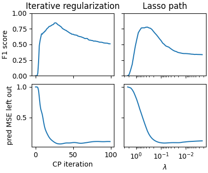
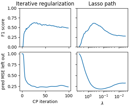
Comparison with Tikhonov in L1 use for support recovery

This example compares Tikhonov and iterative regularization to identify the support of a linear model.

import numpy as np
from numpy.linalg import norm
import matplotlib.pyplot as plt
from sklearn.metrics import f1_score, mean_squared_error
from sklearn.model_selection import train_test_split
from celer.datasets import make_correlated_data
from celer.homotopy import celer_path

from iterreg.sparse import dual_primal
from iterreg.utils import datadriven_ratio

n_samples = 500
n_features = 1_000

The function to compute CP, Lasso path and plot metrics:

def plot_varying_sigma(corr, density, snr, max_iter=100):
    np.random.seed(0)
    # true coefficient vector has entries equal to 0 or 1
    supp = np.random.choice(n_features, size=int(density * n_features),
                            replace=False)
    w_true = np.zeros(n_features)
    w_true[supp] = 1
    X_, y_, w_true = make_correlated_data(
        n_samples=int(n_samples * 4 / 3.), n_features=n_features,
        w_true=w_true,
        corr=corr, snr=snr, random_state=0)

    X, X_test, y, y_test = train_test_split(X_, y_, test_size=0.25)

    print('Starting computation for this setting')

    ratio = 10 * datadriven_ratio(X, y)
    _, _, _, all_w = dual_primal(
        X, y, step_ratio=ratio, rho=0.99, ret_all=True,
        max_iter=max_iter,
        f_store=1)

    fig, axarr = plt.subplots(2, 2, sharey='row', sharex='col',
                              figsize=(4.2, 3.5), constrained_layout=True)

    scores = [f1_score(w != 0, w_true != 0) for w in all_w]
    mses = np.array([mean_squared_error(y_test, X_test @ w) for w in all_w])

    axarr[0, 0].plot(scores)
    axarr[1, 0].plot(mses / np.mean(y_test ** 2))

    axarr[0, 0].set_ylim(0, 1)
    axarr[0, 0].set_ylabel('F1 score')
    axarr[1, 0].set_ylabel("pred MSE left out")
    axarr[-1, 0].set_xlabel("CP iteration")
    axarr[0, 0].set_title('Iterative regularization')

    # last column: Lasso results
    alphas = norm(X.T @ y, ord=np.inf) / len(y) * np.geomspace(1, 1e-3)

    coefs = celer_path(X, y, 'lasso', alphas=alphas)[1].T
    axarr[0, 1].semilogx(
        alphas, [f1_score(coef != 0, w_true != 0) for coef in coefs])
    axarr[1, 1].semilogx(
        alphas,
        np.array([mean_squared_error(y_test, X_test @ coef) for coef in coefs])
        / np.mean(y_test ** 2))

    axarr[-1, 1].set_xlabel(r'$\lambda$')
    axarr[0, 1].set_title("Lasso path")

    axarr[0, 1].invert_xaxis()

    plt.show(block=False)
    return fig


plt.close('all')

When there is noise in the data:

corr = 0.2
density = 0.1
snr = 5

fig = plot_varying_sigma(corr, density, snr, max_iter=100)
fig.savefig("vslasso1.pdf")

# ###############################################################################
# # Really difficult case
corr = 0.8
density = 0.1
snr = 3

fig = plot_varying_sigma(corr, density, snr, max_iter=100)
fig.savefig("vslasso2.pdf")

• 
• 

Out:

Starting computation for this setting
Starting computation for this setting